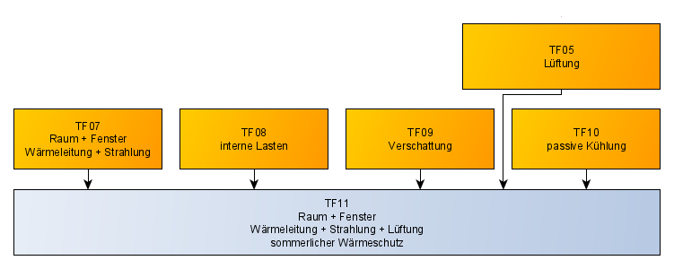
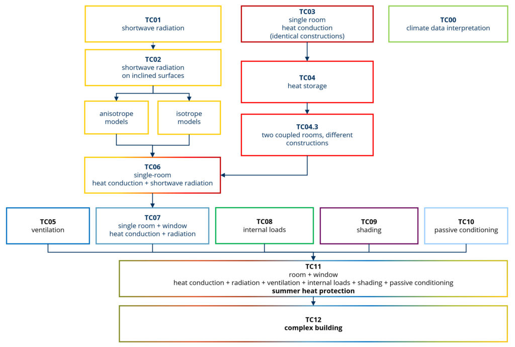
The test cases explained here serve as a validation method of simulation programs. The application scenarios are abstracted to validatable cases. Thus, the simulation program can be checked in the concrete scenario, confirmed or error sources can be found. The following figure provides an overview of the defined test scenarios.
TC01 – Sun Position
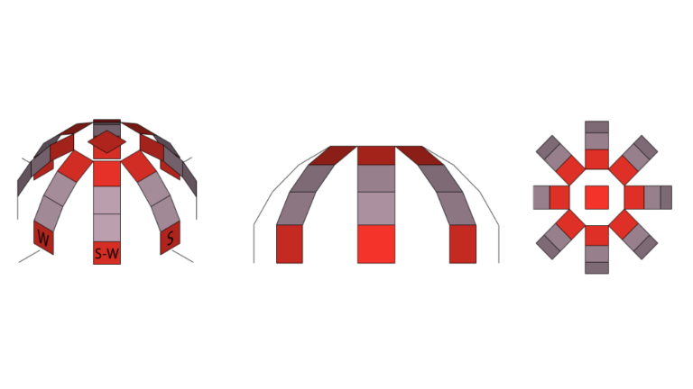
The calculation of the sun position depends only on the time and the location of the building/observer. Therefore, the calculation can also be done independently of the building simulation. Input data are per location: longitude, latitude and time zone. An overview of the selected locations is given in the following figure.

The calculation results are then compared for the following days (March 5, July 27, September 22, October 24, December 17. The calculation results are logged in minute increments on the above days. For each calculation time, both solar elevation angle and azimuth angle shall be given. However, special attention is required for the equatorial azimuth definition in the American context. Detailed information on TC01 can be found in the task description.
TC02 – Solar Gains/Solar Loads
For the calculation of the solar loads in the thermal building simulation, the correct mapping of the radiation intensity onto an (aligned and inclined) surface is necessary. Therefore, for the validation of the radiation load on the building, using determined inclined surfaces. The radiation values are calculated and output at the test location Potsdam.
Basically, there are different models that calculate the radiation on an inclined surface. Here, especially the diffuse radiation is calculated differently. In general, diffuse radiation models for inclined surfaces can be divided into two groups: Isotropic and anisotropic models. These differ in the division of the sky into regions of normal and increased diffuse radiation intensity. The calculation of the radiation load depends on several factors. These include the position of the sun, the climate data, the conversion of the radiation value to the area under consideration, the absorption coefficient of the area under consideration, and the albedo. Further information on TC02 can be found in the task description.
TC03 – Heat Conduction
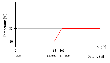
The test case described below is taken from DIN EN ISO 13791 „Thermal performance of buildings“. In this test case, a test room is subjected to a climatic jump in the outside air temperature from 20 °C to 30 °C within one hour. There are a total of 4 test variants in which the layer structure and the material properties of the enclosing structure are changed. In each test variant, all 6 enclosure constructions are of identical design and have the same boundary conditions.
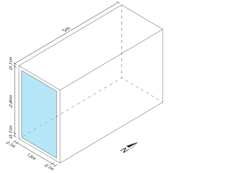
Since the heat capacity of the room air is neglected in this test case, the geometry of the room is secondary and can be changed individually. Further possible combinations of the geometry are described under TC03. For subsequent test cases, the presented geometry of the test room resulted to be advantageous. Note: Unless otherwise specified, this geometry is used in the following test cases. In addition to the geometry, other boundary conditions are also important. The model parameter ventilation, i.e. the air flow rate with the outside air is set to zero. The heat capacity of the room air is also set to zero. Further boundary conditions can be found in the descriptions of TC03.
TC04 – Heat Conduction and Storage
The geometry corresponds to that of Test Case 3, but this time the heat capacity of the room air is explicitly taken into account. Both design setups and climatic boundary conditions are varied, and single-zone models and multi-zone models are tested. Thus, the four following test variants are created and tested:
The TC04 is divided into four test variants. The first test variant is almost the same as TC03 (variant 2) and includes the increase in outdoor temperature in a one-hour interval, taking into account the heat capacity of the air and interior components with increased heat capacity. However, two major adjustments are made. First, the boundary conditions of indoor air is changed. Here, dry air in the room is assumed, where density and heat capacity are changed. Furthermore, three construction elements are now interior walls (N-wall, S-wall, floor) For more details, see TC04.
In the second test variant, heat conduction and storage in different constructions are analyzed under periodic step conditions. In this test variant, all building components are defined as external constructions. Due to the choice of constructions, different surface temperatures occur in the test room. Furthermore, a climate is used which exhibits a periodic temperature jump in order to consider dynamic storage effects. The temperature changes
linearly within one hour. Further details can be found under TC04.
Test variant three includes investigations of heat conduction and storage in coupled rooms under periodic jump conditions. Here, two adjacent rooms with the same room dimensions as in test variant 2, are coupled together. The two rooms are placed side by side in the east-west direction so that an exterior wall of room A faces east, while an exterior wall of room B faces west. The choice of constructions causes a different thermal behavior of the two rooms. For more details, see TC04.
In the fourth and last test variant, the analysis of heat conduction and storage in coupled spaces under climatic boundary conditions is performed. This variant is based on the third test variant . Only the climatic boundary condition is changed. For this purpose, the annual course of the outdoor temperature is used according to the climate data set for the location „Potsdam“. The building is located at a geographical height of H = 81m (this corresponds to 81 m above N H N). Further details can be found under TC04.
TC05 – Ventilation
For the calculation of heat flows between indoor and outdoor air, the correct representation of the air exchange in the thermal building simulation is required. The test case described below tests the functionality of a model or the model implementation/software with regard to the determination of the air exchange between indoor and outdoor air and the resulting energy flows.
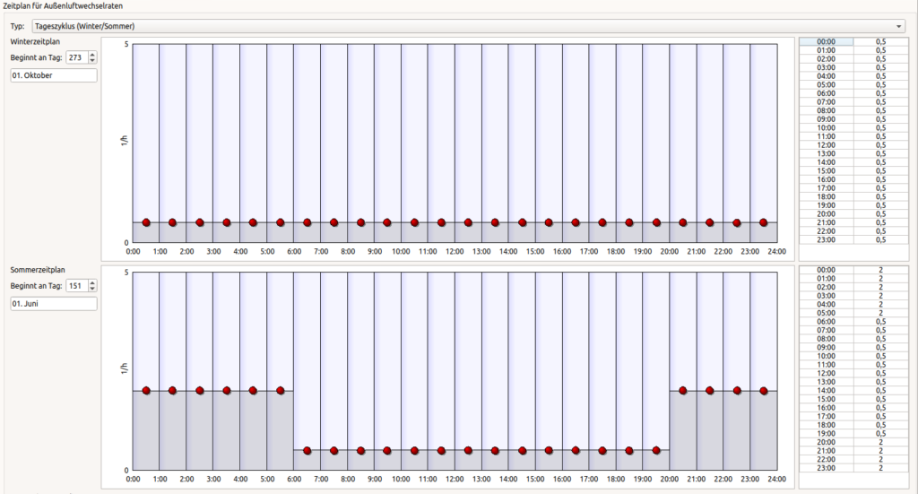
The same construction structure with an insulating layer is chosen on all sides. The thermal insulation property of the insulation layer effectively limits the change of the indoor temperature due to heat conduction through the structure. Thus, the air exchange becomes the decisive mechanism of the indoor air temperature adjustment to the outdoor air. Several test variants are considered, each of which differs in the air exchange rate to be applied. Calculation results of the indoor air temperature (in °C) in hourly steps for the entire year are to be recorded as instantaneous values. Furthermore, it will be checked whether the density of the exchanged air volume is temperature-dependent. Further details can be found under TC05.
TC06 – Heat Conduction and Radiation
For the calculation of the heat balance of indoor air nodes, the correct mapping of the coupled heat conduction/storage with the short-wave radiation is required. The test case described below tests the functionality of a model or the model implementation/software with respect to coupled heat conduction and shortwave radiation. This test case builds on the third test case and is modified by a constant outdoor temperature throughout the year and an adjusted shortwave direct normal radiation. The shortwave direct radiation is constant zero. The air exchange is not considered.
There are also two test variants for this test case. In the first test variant, the constructions have a high storage mass. In the second variant, on the other hand, the components are assigned constructions with a low storage mass. The following calculation results are evaluated in more detail. The first parameter to be output is the temperature of the interior air, as an instantaneous value. Furthermore, the absorbed short-wave radiation intensity of all external surfaces, individually broken down as an hourly integral, is required. For the completion of the test, the convective heat transfer of the interior surfaces, as well as the temperatures of the interior surface of all six components, individually broken down, are also mandatory. Further details can be found under TC06.
TC07 – Windows
For the calculation of the correct heat balance of the indoor air node, the correct mapping of physical effects in windows is necessary. The test case described below tests the functionality of a model or the model implementation/software regarding the determination of the transmitted radiation from windows. For this investigation, a window in the south wall is added to the test room of the sixth test case (see the following figure). Six test variants are created, which are distinguished by different window models.
In the first test variant, only the thermal conduction of the window is examined. The cyclic climate is used, where only one temperature curve exists, all radiation data is given as zero. Further details can be found in TC07.
Test variant two is used to study a simple window model with angle-independent SHGC value. Here, a climate data set is used where non-zero radiation loads exist for the months of July and December. Other constant boundary conditions are an outside air temperature T = 20 °C and Uwindow = 1.1 W/m2K. Longwave radiation through the window is not considered (Tir = 0). Further details can be found under TC07.
The third test variant largely corresponds to test variant two. The only change is the angle-dependent g-value according to the following table. Here, the angle Θ is defined between the sunbeam and the window normal. Further details can be found under TC07.
| Angle Θ | 0 | 10 | 20 | 30 | 40 | 50 | 60 | 70 | 80 | 90 | Hemis |
| SHGC | 0.600 | 0.600 | 0.600 | 0.600 | 0.588 | 0.564 | 0.516 | 0.414 | 0.222 | 0.000 | 0.600 |
In the fourth test case, the window is modeled using a detailed, simple model with the following description. For this purpose, a pane system consisting of
2 float glass panes (each d = 5.7mm) with an intermediate space filled with air (d = 12mm) is modeled. Further details can be found under TC07.
The fifth test variant involves the investigation of a detailed, real window model with low-e coating. This test variant corresponds as far as possible to test variant 2. The modeling of the window is implemented with a detailed, realistic model with the following description. For this purpose, a pane system consisting of a low-e pane and a float glass (each d = 5.7mm) with an interspace filled with argon (d = 12.7mm) is modeled. Further details can be found under TC07.
In the sixth and last test variant, the long-wave radiation of the window is investigated. For this purpose, variant 4 is used as a basis and the radiation climate with long-wave sky counter-radiation is used. Further details can be found under TC07.
For the evaluation of the simulation results, the following calculation results are mandatory. As the first parameter for the evaluation of the simulation models, the temperature of the indoor air as an instantaneous value [°C] is necessary. Furthermore, the transmitted short-wave radiation through the window is required as an hourly average value [W/m2]. Finally, the convective heat conduction through the window as hourly mean value [W/m2] is mandatory. The result data must be determined with at least two decimal places. Further details can be found under TC07.
TC08 – Internal Loads
For the calculation of the correct heat balance of the indoor air node, the correct representation of internal loads such as people, electrical equipment and light is necessary. The test case described below checks the functionality of a model or the model implementation/software regarding the determination of internal loads.
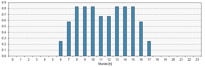
In this test case, internal user loads are applied in the test room. All heat inputs are only entered from February 1, 0:00 hours. Before that, there is no heat input due to the transient phase. The course corresponds to the attendance distribution for a typical office day. The test case is divided into 4 test variants.
In the first test variant, a constant convective heat load is applied with a heat output of PIntLast,Kon = 400 W. In contrast, the second test variant involves a constant, radiative heat load. The heat output is a constant PIntLast,Rad = 400 W. For this, the emissivity of all inner surfaces is set to ε = 1.0. Further details can be found in TC08.
Test variants three and four are the same as variants one and two, but the heat input is based on a schedule. The heat output is controlled according to the table (see above) for both variant three and variant four. In the third variant, the heat output is PIntLast,kon,i = 1000 W · ValueSchedule,i per time step and is entered completely convectively; in the fourth test variant, it is PIntLast,Rnullad,i = 1000 W · ValueSchedule,i per time step and is entered completely radiatively. For this purpose, the emissivity of all inner surfaces is set to ε = 1.0. For more details, see TC08.
The result variables required are the temperature of the interior air, the convective heat transfer of the south wall, broken down to the indoor air node as an hour integral, and the temperature of the interior surface of the south wall. Further details can be found under TC08.
TC09 – Shading
For the calculation of the correct mapping of the radiation loads, the mapping of external shadings is necessary. The test case described below tests the functionality of a model or the model implementation/software with regard to the determination of shading. For this test case, dynamic shading systems such as blinds or shutters are considered in the calculation.
Several test variants exist for this test case as well, in which modeling of non-moving radiation obstructions is performed. These refer to the overhang, the side fin, a combination of the two previously mentioned objects and finally the modeling of a distant body as a single surface. From combinations of these objects, six test variants emerged.
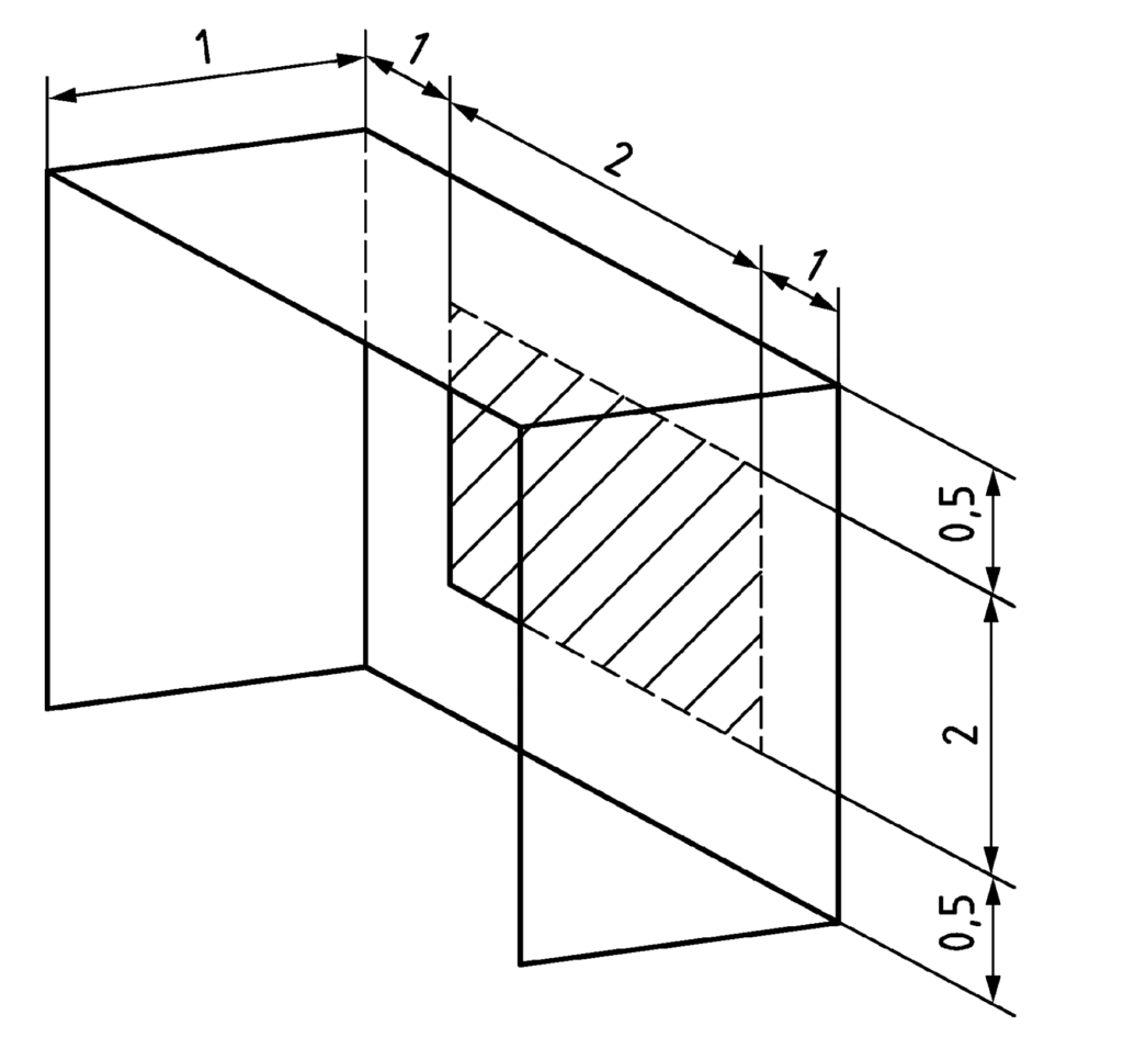
The geometry for the first test variant is composed of 1 m long cantilever, which is 0.5 m above the window. The window is represented by a rectangular profile with dimensions (length x height) 2m x 2m. The wall dimensions are (length x height) 4m x 3m . The cantilever extends the entire length of the wall (4 m). Further details can be found under TC09.
In the second test variant, a south wall with the dimensions (length x height) 4m x 3m and a window located in it with the dimensions (length x height) 2m x 2m is modeled. At each vertical end of the wall there is a fin that cantilevers 1 m perpendicular to the wall and extends over the entire wall height (width x height) 1m x 3m. Further details can be found under TC09.
A combination of test variants one and two represents the third test variant, whose geometric representation can be seen in the figure above. In the following variant four, the shading of a south-facing wall is done by an external obstacle. In this case, a significantly larger obstacle is placed in front of a south-facing wall, at a distance of 5 m. The obstacle is placed in front of the south-facing wall. Further details can be found under TC09.
Only one change in alignment occurs in test variants five and six. Based on the third test variant, the orientation changes to the east (orientation 90 °) in the fifth test variant. Variant six is based on the fourth variant. Equivalently, only the orientation of the walls is adapted to the east.
In the last variant, dynamic shading is considered, which is controlled by a global radiation sensor. As calculation results the sun direction angle (azimuth), the sun elevation angle (altitude) and the sunlight factor of the shaded area shall be considered. The geometry of Test Case 7.1 is adopted as the test space. At an intensity of 150 W/m2 on the south facade, the shading becomes active. There is no time delay in activating the shading. For this purpose the weather of Potsdam including an associated location is used for the calculation of the sun position. Further details can be found under TC09.
TC10 – Passive Cooling
For the calculation of the correct heat balance of the room air node, the correct mapping of thermal conditioning components in the room is necessary. The test case described below tests the functionality of a model or the model implementation/software with respect to determining the thermal balances of conditioning systems.
For this test case, an underfloor heating or cooling system is assumed and convective and radiative heat transfer are considered. A test and a real climate data set are used. All elements, including ceiling and floor, are identical (same material parameters and layer sequence) and have the same boundary conditions. Six different test variants are given.

n the first test variant, the room is conditioned by pure convection heating or cooling. Here, the analysis of the ideal (air) conditioning is carried out. Predefined schedules for the room setpoint temperatures of heating and cooling are used as a basis. Long-wave radiation exchange of indoor surfaces is not considered. Maximum heating power is limited to 500 W and maximum cooling power to 300 W. Further details can be found under TC10.
The second test variant includes a layer in the floor with a detailed surface conditioning model. This test variant is designed to evaluate an underfloor heating and cooling system with convective heat transfer. In addition to the parameters already described, other boundary conditions are necessary. These include the non-consideration of the long-wave radiation exchange through interior surfaces, as well as a schedule-controlled flow temperature. Further details can be found under TC10.
Based on the second test variant, only an adjustment of the long-wave radiation exchange of the interior surfaces was made in the third test variant. Here, the emission coefficient ε = 1 is set. Thus, the long-wave radiation is completely absorbed. Further details can be found under TC10.
The template for test variant four is test variant two. There is an exchange of the climate data set, and a thermostatic valve is also introduced. The thermostatic valve is controlled on the basis of the room air temperature. The setpoint is set to a constant 20 °C and the supply temperature is modified. The year is divided into two periods. The first period extends from 01/01. – 16/08. of the simulation period, whereby the flow temperature is given a constant value of 35 °C. The second period begins accordingly from the beginning of the simulation period. Accordingly, the second period begins from 17.08. Starting with the second period, the conditioning of the supply temperature of a typical heating curve, mathematically formulatable by: TV L = max (21 °C, min (35 °C,-0.5 – Tout + 30 K)). For more details, see TC10.
Based on the fourth test variant, only an adjustment of the long-wave radiation exchange of the inner surfaces was made in the fifth test variant. Here, the emission coefficient ε = 1 is set. Thus, the long-wave radiation is completely absorbed. Further details can be found under TC10.
For the sixth test variant, test variant four again serves as a template. All parameters are taken from it and adjustments, respectively changes of the climate data set and the exchange of the longwave radiation at the inner surfaces are made. For more information on the climate data set, see TC10. By changing the emission coefficient ε = 1, the long-wave radiation is completely absorbed. In addition, a thermostatic valve is introduced. The thermostatic valve is controlled according to the room air temperature. The set point is set to a constant 24 °C. The flow temperature is also modified. The supply temperature follows a cooling curve with the following mathematical formulation: TVL = max (18 °C, min (24 °C, -0.5 – Tout + 36.5K)).
The analyses focus on the following results. The first parameter to be evaluated is the temperature of the indoor air as an average value [°C], followed by the averaged return temperature of the fluid [°C] from test variant two onwards. Furthermore, the indoor surface temperatures of floor and ceiling, as mean values [°C], as well as convective heat input or extraction at the indoor air nodes and convective heat transfer across the floor surface are required for the evaluation of the simulation tools. For more details, see TC10.
TC11 – Summer thermal protection
For Test Case 11, Summer Thermal Protection, a combination of five complex previous test cases is performed. Ideal heating and cooling (Test Case 10), a window (Test Case 7), shading (Test Case 9), air changes (Test Case 5) and internal loads (Test Case 8) are applied. In addition, two different climate data sets are tested.